 |
Links : Home Index (Subjects) Contact StatTools |
|
Related Links:
All mathematics involves the transformation of one set of numbers to another set, but transformations provided by StatTools are those commonly used in clinical statistics.
Data Input :
Transform to a new minimum (min) and maximum (max) as nominated by the user, uses the following formula
Transform to a new mean (mean) and Standard Deviation (sd) as nominated by the user, uses the following formula
Transforming to new minimum/maximum or new mean/Standard Deviation provides a new numerical scale, but do not change the relationship between the values. Ranking is frequently used in non-parametric statistical calculations, and in many instances, it is used to constrain outliers, to bring the distributions closer to that of normal distribution. The values are ranked in ordered, and replicated ranks are averaged. The ranks can be ascending or descending in order.
Introduction
Logarithm
Power
Box Cox
Poisson Related
Proportion or Probability Related
Polynomial
Transformation may produce values which have a curvilinear relationship with the original. This is commonly required in
the handling of data in the biomedical domain.
A common reason for a curvilinear transformation is to follow the natural relationship between two measurements. For example :
Another reason for a curvilinear transformation is for measurements with natural closed ended constraints. For example, proportions have a range of 0 to 1, Poisson distributed counts have a minimum value of 1, and ratios have values exceeding zero (0). When the range of measurements in a particular analysis is distant from the natural constraints, such as a proportion around 0.5 and counts exceeding 30, the measurements can be analysed as if they have an infinite range, as the confidence intervals would not impinge or overlap the constraint values. However, when the range is close to the natural constrains, such as a proportion <0.05 or >0.95, or a count close to 1, the confidence intervals calculated many impinge upon or even overlaps the constraint value, making any reasonable By far the most common reason for a curvilinear transformation is to convert measurements that are not normally distributed to one that is, so that the powerful and user friendly parametric statistical procedures can be used for analysis. Three common types of distribution are common in biomedical analysis, and difficult to handle, and these are :
Natural logarithm (y = loge(x), x = ey) is commonly used in preparing data for parametric statistical analysis.
This transformation should be used for any measurement that is a ratio, when there is a positive skew in the data (long
tail on the right hand side). In fact, in many biological measurements that are not initially normally distributed,
a logarithmic transformation renders the data normally distributed.
Values for logarithmic transformation must be >0 Natural antilogarithm or exponential transformation (y = antiloge(x), y=exp(x), y = ex) is the reverse of the natural logarithm. This transformation is used at the end of an analysis using log transformed values, to convert the results to the original units of measurements. Value for exponential transformation can be both positive and negative values. However very large value may exceed the limit of calculation and crash the program. Logarithm with a nominated base produces similar results as the natural logarithm, except that numerically they are scaled differently. Based logarithm, especially the use of base=10, is favoured by clinicians as the results are intuitively easier to interpret (1=10, 2=100, 3=1000, etc). The formula is
Antilogarithm with a nominated base is used at the end of analysis that used the based logarithmic transformed values, to reverse transform the results to the original measurement units. The formula is
Value for based antilog transformation can be both positive and negative values. However very large value may exceed the limit of calculation and crash the program. Power transformation (y = xpower) is a flexible and powerful tool to change distributions of a set of data. A power value of <1 uses roots, so tends to move the skew to the left, while power value >1 moves the skew to the left. The range of positive and negative power values produce different curved relationships between the original (x) and transformed (y) values. The square root transformation (y=x0.5 is a special case of power transmission, and it is sometimes used in data that have a geometric distribution. A typical case is the measurement of discrete periods, such as the number of operations between complications, number of minutes in waiting time, especially if these periods are close to 1.
The Box Cox transformation was originally devise to transform time to events to a normally distributed measurement for analysis,
the arguments surrounding its use are as follows.
Reverse transformation : y = exp(x) if λ=0, otherwise y = {xλ+1)1/λ This leaves the question of which λ to use. In many cases, the correct λ can be found in similar work published, as comparison of results requires that the same transformation is applied. When there is no suitable existing λ values, then a value that will best transform the data to normally distribution should be used. The following criteria are used to determine the closeness a transformed data set is to normal distribution.
Please Note : The author came across the following transformations while researching the Box Cox transformation, and thought these may be of interest or useful to some users. The author has no experience in using these transformations.
When dealing with Poisson distributed counts, researchers may use the reverse of a Poisson Count (1/λ) to analyse data, as this is a continuous measurement that can be transformed into a normal distribution. The impetus for developing a direct transformation for the Poisson distributed count comes from radio-active scanning, particularly that of Positron Emission Scanning, where the image received consists of pixels, each one of which is a count of emission. Given that the Poisson distribution is asymmetrical on the two sides of the mean, with a very long right tail, there is a need to transform counts into a normally distributed measurement, so that de-noising algorithms can be applied. The Freeman-Tukey Transformation is an approximation of the square root transformation, with an adjustment for low values. The formula is y = sqrt(x+1) + sqrt(x). With high count values, x+1 is approximately the same as x, so the transformation is effectively 2sqrt(x). The Anscombe Transformation is also a variant of the square root transformation, where y = 2sqrt(x + 3/8). As the value of x increases, the 3/8 addition becomes increasingly trivial, so that, with very large counts, the transformation is approximately 2sqrt(x). The interesting part of Anscombe is the reverse of the transformation, as the asymmetrical and unstable variance returns when the results are reverse transformed into counts. Three variants of the reverse transformation are therefore offered.
 Proportion or probability are increasingly being used as a measurement. Examples are the probability that a baby is genetically
abnormal, or the risk level of complication for a surgical procedure.
Proportion or probability are increasingly being used as a measurement. Examples are the probability that a baby is genetically
abnormal, or the risk level of complication for a surgical procedure.
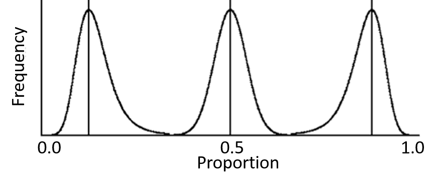
Although proportion is a continuous measurement, it is close ended, with a minimum value of zero (0) and maximum of 1. It follows the binomial distribution, which is similar to the normal distribution when the sample size is large and the value near 0.5. As the sample size decreases so that its variance increases, or that the value approaches the extremes of 0 or 1, its natural variance, measured as the Standard Deviation, becomes increasingly asymmetrical, as shown in the diagram to the left. Many statistical procedures treat proportions as if they are normally distributed, and this works reasonably well in most cases. However, if the sample size is small, or the value close to the extremes of 0 or 1, the confidence interval overlaps the 0 or 1 value, creating a conceptually inconceivable situation, and produces a flawed conclusion. There are two commonly used transformation to create normally distributed measurements from proportions or probability.
In the bio-medical domain, there are many curvilinear relationships that do not follow precise mathematical formulation, and these
must be established by empirical observations and comparisons. A common algorithm to do so is polynomial curve fitting, where
y = a + b1x + b1x2 + b3x3 .... and so forth, although in biology,
polynomial coefficients beyond the third power have very little practical implication, and are therefore seldom used.
Biochemical laboratory uses curve fitting extensively in translating observations in a test, such as radiation counts, color depth, light absorption, to concentration of substances they are measuring. Curve fitting is also used clinically, often to predict outcome, a common use in obstetrics being to nominate the average birthweight or an ultrasound measurement from the gestational age. StatTools provides a curve fitting program in the Curve Fitting Program Page , which allows curve fitting to the fifth power, far in excess of most requirements. Results for such curve fitting, or formula obtained from published work, can be used to transform data accordingly in the Numerical Transformation Program Page
Introduction
Fuzzy Logic
The miscellaneous section is used to contain all those transformations that may be useful, but do not belong to any specific
classification. Although these are few currently, it is expected that more will be added as StatTools continues
to expand in response to user needs.
The concept of fuzzy logic was explored by the department in the early 1990s, when there was an interest in using the neural
network to establish a system of machine based decision making. Because the fuzzy logic transformation is useful, it is retained
and continued to be used as a statistical transformation, when the department's interest in machine based diagnosis waned.
Fuzzy logic uses the mathematics of probability to define truth. In other words, it sees true and false merely as extremes, when reality is somewhere in between. Fuzzy logic therefore uses the principle of logistic transformation to convert any measurement into degrees of certainty with a value between zero (0) and one (1), where 0 is absolute certainty for negative, and 1 absolute certainty for positive. Fuzzy logic transformation is also commonly used to transform a continuous measurement into a bimodal distributed conclusion. Thyroxine levels are transformed into probability of thyrotoxicosis, temperature readings into fever, pH into acidosis or alkalosis, PO2 into hypoxaemia, and so on. The basic logistic formula is p = 1 / (1 + exp(-v)), where v is value ranging from -∞ top +∞, and p is probability ranging from 0 to 1. There is no difficulty in interpreting probability (p) as level of certainty, but the range of v varies from -∞ to +∞, so the main issue in fuzzy logic is how to scale the measurement value x into a convenient parameter v to be used in the logistic equation. The algorithm is as follows

We wish to have an indicator for the health of the new born by measuring it's umbilical cord blood pH, and set the following criteria
By changing the values vlow and vhigh, users can define ranges of values that can be interpreted as positive, negative, and varying level of uncertainty. The program in the Numerical Transformation Program Page allows these parameters and the data to input by the user, but fixed the Plow to 0.05 and Phigh to 0.95. The table to the right provides logit values for different p values, which the users can use if he/she requires decision levels other than p=(0.05,0.95) |
 |