This section supports the program in the Sequential Paired Difference Analysis Program Page , where differences between pairs of measurements are evaluated sequentially against the null hypothesis (that the mean of the difference = 0). Evaluation takes place after each pair, and a decision is made to reject the null hypothesis (significant difference exists), to accept the null hypothesis (no significant difference), or to continue to collect data.

Two models are available. The first assumes that the variance (standard deviation) is known, and this is incorporated into the parameters. The second accepts that the variance is not known, and the mean and standard deviations assigned are merely used to define the effect size (difference / standard deviation) that the model can work with.

The parameters that needs to be set are as follows.

• Probability of type 1 error alpha (α), the default is usually 0.05 for one tail. If a two tail model is preferred, the α value used should be halved, as α_{two tail} and 2α_{one tail} produce the same numerical results.
• Power (1 - β). For most clinical studies this is set to 0.8, but most of the examples set in Armitage's book set this at 0.9 or 0.95.
• The difference and standard deviation of that difference. This defines the effect size which the model is to detect. The smaller the effect size, the larger will the sample size be before a decision can made.

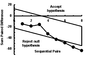
Border y = a + bx b = -4.0 a (reject null hypothesis) a = -22.18 a (accept null hypothesis) a = 12.47 Maximum n for restricted model = 8

We wish to evaluate whether two methods of measuring blood pressure. We suspect that the mercury manometer(A) would have a lower reading than the electronic (B) one, and wish to test if this is true. We therefore adopted the one tail model, which is the default setting for the program.

We set the parameters as alpha (α) = 0.05 (one tail), power=0.8. We are only interested if the difference is large (1 standard deviation), so we set the difference to be detected as -8mms, and the expected Standard as 8mms Deviation of the difference, both at 8mmHg.

Pairs	A	B	diff(d)	Sum(d)
1	80	95	-15	-15
2	120	124	-4	-19
3	75	72	3	-16
4	75	92	-17	-33
5	84	94	-10	-43
6	100	106	-6	-49
7	88	96	-8	-57
8	92	98	-6	-63

The borders are :

• The border for rejection of null hypothesis is y = -22.18 - 4x, and for acceptance of null hypothesis y = 12.47 - 4x, if BP_A<BP_B
• Where x = sequential pairs, and y = sum of differences.
• If the borders are not crossed after 8 pairs of measurements (maximum), the null hypothesis is accepted (no significant difference)

The data are shown above and to the right. A is the BP as measured using the mercury manometer and B that measured electronically.

Although the data is evaluated after each subject, the graph to the right shows all the results after 8 subjects are evaluated.

The borders for rejection and acceptance of the null hypothesis, and the truncation after 8 pairs, can be seen. The slopes are downwards because measurements A are consistently less than that of B.

The redundant coordinates are edited out, and the graph rescaled , resulting in the final plat as shown to the right.

Althpugh 8 pairs of differences are shown, decision could have been made after the fifth pair, that the mercury manometer (A) produces a significantly lower measurement than the electronic manometer(B).

In the variance unknown model, the effect size (difference / SD) can be used, so that the Standard Deviation can be set to the value of 1, and the difference to be detected set to the value of the effect size. When there is no precise value available, the following conventions are often used.

• An effect size (difference/SD) of 0.3 or less is considered a small effect, and are rarely used in sequential studies
• An effect size of 0.7 or more is considered large enough to be obvious, and these are most commonly used, particularly in drug trials
• Effect sizes between 0.3 and 0.7 or moderate size are common in clinical situations, and can be (but not that commonly) used in sequential analysis.

n	A	B	diff(d)	Sum(d)	Sum(d2)	z
1	80	95	-15	-15	225	1
2	120	124	-4	-19	241	1.5
3	75	72	3	-16	250	1.0
4	75	92	-17	-33	539	2.
5	84	94	-10	-43	639	2.9
6	100	106	-6	-49	675	3.6
7	88	96	-8	-57	739	4.4
8	92	98	-6	-63	775	5.1

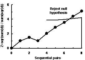
We used an effect size of 1.0 for this example, the same as a difference of 8mmHg when the Standard Deviation is 8mmHg.

The results of calculations are presented in the table to the right, with a truncation at 7.9 (rounded to 8) pairs.

The sequentially calculated effect is calculated from the cumulative difference of the pairs (d), where z = sum(d)² / sum(d²). This z value is matched against the decision criteria, the values of which have a hypergeometric distribution, and are are calculated as the sample size increases.

If z fails to cross the decision line by the calulated maximum of 7.9 pairs (ie. 8 pairs), then the null hypothesis is accepted.

The table above and to the left shows how the z value is calculated, and the results are plotted in the diagrm to the right.

The results show that the rejection border has been crossed by the seventh pair, and at that time the conclusion that a significant paired difference exists could be drawn. At the seventh pair, the sum of differences is -57, an average of -57/7 = 8.1. The conclusion at this point is that the mercury manometer measures blood pressure on average 8mmHg lower than the electronic manometer, and this difference is statistically significant.

Please note : As the variance unknown model is mostly used when the precise background parameters are not available, the main interest is to detect a difference in either direction, so a two tail model is usually used. This example uses a one tail model to remain consistent with the default one tail setting for both known and unknown variance. If the two tail setting is chosen, the decision to reject the null hypothesis would be made at the 8th pair and not the 7th pair.

This section is related to the Sequential Paired Preference Program.

In the sequential preference analysis model, pairs of responses are evaluated as preference for the first response (a), represented by +1, or preference for the second response (B) represented by -1. If the response is tie or neutral, the value is 0, and ignored by the program.

The following examples demonstrate this model.

• Two treatment for headache are tested on the same individual at different times, aspirin (A) and paracetamol (B), and the patient is asked which treatment relieves pain better. The data is +1 if A (aspirin) is preferred, and -1 if B (paracetamol is preferred). The data is 0 if the respondant cannot decide which is better.
• In matched pairs of women admitted for elective Caesarean Section, one is given a prophylactic antibiotic (A) and the other not given prophylactic antibiotics (B). If A develops post-operative infection and B does not then the data is +1, If B develops post-operative infection and A does not then the data is -1. If both have the same post-operative progress then the data is 0.
• Women leaving the hospital after child birth are asked whether they are satisfied with the care and attention they received. Those satisfied score +1 and those dissatisfied score -1. Those with neutral or no response score 0.

The data is therefore a single column of +1, -1, or 0. Zeros (0) can be left out as the program does not include zero values in calculation. The sums of the values are tested against the null value of 0 after data from each pair is collected, usinf decision borders to determine whether to stop the study and reject the null hypothesis, to stop the study and accept the null hypothesis, or to continue data collection.

The decision borders are calculated using the following parameters

• Probability of type 1 error alpha (α), usually 0.05. The program from Sequential Paired Preference Analysis Program Page provides a default one tail model for decision making. If a two tail model is required, the α value should be halved, as α_{one tail} and 2α_{two tail} produces the same results.
• Power (1 - β). For most clinical studies this is set to 0.8, but most of the examples set in Armitage's book set this at 0.9 or 0.95.
• The expected proportions of preference for the two options (p1, and p2), to calculate the effect size for the model.

The results produced are the border coordinates and the plotsw, as demonstrated in the example.

1
1
1
-1
1
1
1
1
-1
1
1
1
1

We wish to compare two headache pills (A and B). We set our parameters so that alpha = 0.05, power = 0.9, The model should be able to detect a difference where preference for one pill is 70% (0.7) and preference for the other is 30% (0.3).

From preliminary data we expect pill A to be better than pill B, and we widh to confirm this, so the one tail model is used, and the probability of Type I Error for statistical decision is set to α = 0.05. We also follow the example set by Armitage's book and use a power of 0.9

Effect size θ = 0.8448 Rejection border : y = 3.4113 + 0.3809 x Acceptance Border : y = -11.606 + 1.0961 x Maximum number of pairs for truncation = 21

The border to decide rejection of the null hypothesis is shown to the left, being y = 3.4113 + 0.3809 x, and if this border is not crossed after 21 pairs, then the null hypothesis will be accepted (no significant difference).

As each subject report his preference, the no preference response is ignored (either not included into the data array or, if included will be ignored by the program). Those preferring pill A will be scored 1 and those preferring pill B will score -1, and the scores are summed and plotted on the graph.

Although a decision is made after each subject, the data presented above and to the left represents that obtained after 13 subjects, and the plot at that time is as shown to the right.

It can be seen that, the border is crossed after 12 subjects have been provided their preference, and the null hypothesis can at that point be rejected (significant difference shown). Also that, being a restricted model, the study is truncated at 21 pairs, and the null hypothesis is accepted (no significant difference) if the border is not crossed after 21 subjects.

At the end of the plot, excess lines are removed and the plot rescaled to make the results clearer.